Spectrophotometry as an Analytical Tool
Light is a form of energy. In scientific terms, it can be described in two ways: (1) electromagnetic radiation, or light waves, and (2) particles of energy, known as photons. The light wave is comprised of an electric field (E) and a magnetic field (H), which travel through space at right angles to each other. The wave is created by the acceleration of some charged particle, such as an electron. The acceleration of the particle induces the electric and magnet fields which travel away from the charged particle as a light wave.
A light wave is described by a number of characteristics: wavelength, frequency, velocity, and amplitude. The wavelength (λ) is the distance between two consecutive wave peaks. The frequency (v) is the number of complete wave forms (wavelengths) that pass a point in space in a period of time. The velocity of light through any homogeneous medium is constant. Consequently, the frequency and wavelength of a light wave can be related by the following equation:
velocity = λv
The velocity of light in a vacuum (c) (3.00 x 10⁸ m/s) is commonly used in scientific calculations of frequency and wavelength, giving:
c = λv
Finally, the amplitude (a) is the height of the wave and is related to the intensity of a light beam.
When light is described as “particles of energy,” the smallest definable particle is the photon. The energy of a photon (E) is dependent on the frequency of the light and can be qualified by the following formulas:
E = hv or E = hc/λ
where h is Planck’s constant (6.62 x 10⁻³⁴ J-sec). This relationship illustrates two important points: that light of a particular wavelength (or frequency) is quantized – that is, it has a single energy value at that wavelength; and that light can be used as a source of quantized energy in the study of chemical systems. It is important to note that energy and wavelength are inversely proportional: short wavelength light has higher energy than longer wavelength light.
If you could physically “grab” a light wave and stretch it to make its wavelength slightly longer, you would also change the energy level of that light, as related by Planck’s equation. Every light wave has a specific wavelength, and each wavelength has a corresponding energy level. There is a relatively small region called “visible light” that includes the range of energies with which the molecules in the retina of our eyes interact in order to transmit visual images to our brain. Our eyes are capable of sensing only a very small portion of the entire electromagnetic spectrum! Similarly, a radio receiver cannot sense visible light, although it can interpret much longer wavelength (lower energy) radio waves.
Matter is composed of particles (neutrons, protons, electrons, atoms, molecules, etc.) that are held together by a variety of forces. Neutrons and protons are held together in the nucleus of an atom by very strong nuclear binding forces. Electrostatic forces hold electrons in specific energy levels around the nucleus. Atoms are bonded to each other by forces of attraction within certain allowed energy levels, depending on the nature of the atoms. All of these forces help to define a world in which different particles are held in specific energy levels relative to each other. Each level has a single energy value and is, therefore, quantized.
The energy associated with each of these levels depends on the type of particles being held together. The energy levels of nuclear forces are higher than those of the electrostatic forces that hold electrons in orbit around the nucleus. Even lower energy levels are associated with the bonds between atoms and molecules, while very low energy levels are required to rotate molecules in space.
For most of these particles, there is more than one quantized energy level in which the particle can exist. For example, the outermost electron in a sodium atom normally resides in a 3′ orbital, its lowest possible energy level (or ground state). This electron can, however, be excited to an empty 4p orbital, if the atom absorbs the amount of energy exactly equal to the energy difference between the two orbitals. It is this phenomenon that forms the basis of absorption spectroscopy
When matter interacts with an energy source (heat, sound, electricity, light, etc.) some of the energy can be absorbed, causing the particles to be elevated to different energy levels. In some cases, the particles can be excited totally out of the original chemical system holding them in place. This is what happens when sugar absorbs heat energy, which causes the sugar molecules to decompose into carbon dioxide and water. Under certain conditions, though, the amount of energy absorbed can be controlled, and information about the chemical system can be obtained. This is the case in absorption spectroscopy. The table below lists the types of changes that occur during the light absorption process in regions of the electromagnetic spectrum.
| Wavelength Region | Wavelength Limits | Types of Transitions in Chemical Systems with Similar Energies |
|---|---|---|
| Gamma ray | 0.01 – 1 A | Nuclear proton/neutron arrangements |
| Ultraviolet | 10 – 380 nm | Outer-shell electrons in atoms Bonding electrons in molecules |
| Visible | 380 – 720 nm | Same as ultraviolet |
| Infrared | 0.72 – 1000 µm | Vibrational position of atoms in molecular bonds |
| Microwave | 0.1 – 100 cm | Rotational position in molecules Orientation of unpaired electrons in an applied magnetic field |
| Radiowave | 1 – 1000 m | Orientation of nuclei in an applied magnetic field |
The Absorption Spectrum
If we monitor a beam of light shining through a sample containing a substance that can absorb one of the beam’s wavelengths, we can obtain a plot of the amount of light absorbed versus the wavelength, as shown in Figure 1a. This plot is known as an absorption spectrum, and shows which particular wavelengths of light a chemical species can absorb. The energy associated with the absorbed wavelength corresponds to the energy difference between the electronic levels involved in the excitation of the electrons in the absorber. In solution, these energy levels are modified by the properties of the solvent. Subsequently, they can have a number of different energy values. Thus, when we repeat the experiment with a molecule or ion in solution, many different wavelengths adjacent to the main transition wavelength are also absorbed. This is shown in Figure 1b.
Figure 1: Absorbed Light vs. Wavelength
The absorption spectrum for a substance can be used to identify the presence of that substance, since every chemical species has a specific set of energy levels that it can absorb, depending on its unique electronic configuration. Unfortunately, the levels of these species in solution are modified so greatly that many different substances assume similar levels. Thus, the absorption spectra for many compounds and ions look the same.
Quantitative Measurements
A primary use of absorption spectroscopy lies in its applicability to quantitative measurements. This is a function of how much light is absorbed, and how that relates to the amount of the absorber present in the sample. The following derivation presents the basics of this relationship.
When we shine a light beam of a certain wavelength (l) and initial intensity (I 0 ) through an absorbing sample contained in a spectrophotometer cell, the intensity of the light beam transmitted through the sample (I t ) is dependent on three factors (see Figure 2). The first factor is whether the sample will absorb light at that wavelength. The second is the amount of sample which the light must pass through or, the cell width (b). The third factor is the concentration of the absorbing species in the sample solution (C). You can see through a test tube containing micromolar concentrations of the same species. The fraction of light transmitted, or transmittance (T), is defined as the following:
 (1)
(1)
and,
 (2)
(2)
where,
The transmittance of the sample varies logarithmically with the cell width and the concentration of the absorbing species in the following way:
 (3)
(3)
The proportionality constant depends on the chemical nature of the individual absorber, the wavelength at which the measurements are being made, and the units of b and C. In visible absorption spectroscopy, b is normally measured in centimeters. If C is also measured in mol/L (molar concentration, M), the proportionality constant is defined as the molar absorptivity (ε), which has units of l/M-cm. If C is measured in any other units (e.g., g/l), the constant is simply called the absorptivity (a), whose units will depend on C. Under normal operating conditions, ε or a is determined experimentally by measuring a standard of known concentration.
Figure 2: Factors that Determine Transmitted Light Intensity
Beer’s Law
The relationship on the preceding page relates the amount of light transmitted through the sample to the concentration and cell width. We frequently like to think in terms of how much light is absorbed by the sample, so we define a new term, absorbance (A):
 (4)
(4)
Making all of the appropriate substitutions, we get:
 (5)
(5)
or,
![]() (6)
(6)
This equation is known as Beer’s Law, which shows the linear relationship between the absorbance and the concentration of the absorbing species. In chemical analyses, the following three methods can utilize Beer’s Law:
- Absolute Calculations
Absorptivity or molar absorptivity is calculated by measuring the absorbance of a standard of known concentration in a cell known cell width. This calculated value is then used to determine an unknown concentration of the same absorbing species from the absorbance measurement at that concentration.
- Working Curve Analysis
The absorbance of a series of three to five standard solutions are measured and plotted on graph paper against the concentrations of these standards. This is known as a Beer’s Law plot. The absorbance of an unknown concentration is then measured, and its concentration is determined directly from the plot. This method is more commonly used than the absolute calculation, because experimental error will average out over the number of standards.
Figure 3: Beer’s Law Plot
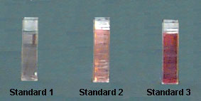
Figure 4: Example of change in color as concentration of solution increases.
3.Standard Addition Analysis
This method is used when certain matrix interferences may cause problems with the measurements. The assumption is that the interference will act equally on the analyte and on an standard added to analyte. In this case, the sample is measured (A1), and then a second portion of the sample is spiked with a standard and this is measured (A2).
We will use the first two methods in the laboratory experiment.
To measure the absorbance of light by a sample, we use an instrument called an absorption spectrometer (or spectrophotometer). The basic components of the instrument are shown below. In the visible light region, a common white light bulb (similar to those found in high intensity desk lamps) is used as the light source. In the UV region, a deuterium lamp is used. To isolate the wavelength of interest from all of the others coming out of the bulb, we reflect the light off a grating, which disperses each wavelength of the light beam at a different angle. By controlling the angle of deflection, we can get the proper wavelength to pass through the sample cell into a light detector (phototube). The phototube contains a cathode coated with a substance which will emit electrons when it is struck by photons. The electron current is measured by a meter or a digital readout.
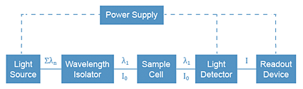
Absorption Spectrophotometer Components
In lab, we will use the Spectronic® Genesys 5 spectrophotometer made by Milton Roy.
How to Use the Spectronic® Genesys 5
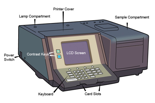
Front View of the Spectronic Genesys 5
Main Keyboard of the Spectronic Genesys 5
Main Keyboard Key Functions
| Name of key | Function |
|---|---|
| ACC | Sets parameters (e.g., auto increment, temperature) used to control the automated accessory currently installed in the instrument |
| AUTO ZERO | Sets the instrument to 0.0A or 100%T |
| CELL (up arrow) | Increments the Multi-Cell Holder one position (from position #8, the holder will advance to position #1) |
| CELL (down arrow) | Decrements the Multi-Cell Holder one position (from position #1, the holder will advance to position #8) |
| CLEAR | Clears the numeric or alphanumeric entry field, one character at a time |
| CONTRAST | Controls the contrast of the display |
| ENTER | Accepts the displayed entry |
| EXIT | Backs up one screen in the software or out of the screen currently displayed. Pressing the key causes the instrument to accept any valid changes made. |
| GO TO WL | Sets the analytical wavelength |
| MINUS (-) | Used for numerical entries |
| NUMBER KEYS | Used for numerical entries |
| PERIOD (.) | Used for numerical entries |
| Sends screen information or test results to the selected printer (internal or external to the instrument) | |
| SAMPLE ID | Sets (changes and enters) a new sample identifier (alphanumeric) |
| SETUP TESTS | Accesses the application program set-up screen, enabling you to enter instrument and test parameters for the current test |
| TEST TYPES | Loads a specific test, previously stored, from a Memory SoftCardTM or from the instrument (default test) |
| UTILITY | Accesses selected instrument functions (lamp interchange wavelength, time/date settings, language, turning lamps on and off, printer / plotter devices, parameters for RS-232-C port) |
View a video demonstration on how to use a spectrophotometer